Following on from Part 1 of this series (Part 3 available here), this article aims to build on other analytical techniques commonly used within medical research, focusing on simple examples.
Probability and testing
Before exploring hypothesis testing, it is vital to understand the basics of probability. The term probability is used to describe a numerical measure of the chance of a particular event occurring or the frequency of the event occurring. It is commonly written as a percentage or a decimal; for example, 20% is depicted as 0.2 as a decimal.
Therefore, 100% (1.0 in decimal) means that there is a guaranteed chance that an event will occur, while 99% (0.99) means that it is not guaranteed, yet a very high possibility is still present. Hence, probability can only lie within the range of 0% to 100% (or 0 to 1.0). It is now common to say that probability is a degree of belief in an event occurring, rather than objectivity that an event will occur (as it is not possible to have objectively observed the frequency of an event occurring in a particular reference group) [1].
The events themselves can be classified as independent or mutually exclusive. Consider two events; if these are independent, they can occur at the same time and are thus unrelated. While mutually exclusive events cannot both occur at the same time [2]. If we were to work out the total probability of two mutually exclusive events occurring, we take the sum of the probabilities of the events. On the other hand, if the events are independent, then we must take the product of the probabilities instead.
Probability values that are used to test a hypothesis, a suggested theory that we are working to prove or disprove, are depicted as the P value. First, we form a null hypothesis and an alternative hypothesis. The null hypothesis states that there is no significant difference between populations or groups that are being investigated. For example, suppose we are testing the probability of picking a blue ball out of a bag containing blue and red balls. The null hypothesis would state that there should be an equal chance of picking out blue and red balls and thus there is no significant difference in the likelihood of each event occurring. This is denoted as: H0 = probability of picking a blue ball is 0.5.
The alternative hypothesis, on the other hand, states that there is a significant difference in the likelihood of each event occurring. In this example, the alternative hypothesis, denoted as HA, could be as follows: HA = the probability of picking a blue ball is lower.
Continuing this example to understand the P value, say we pick a ball 600 times; using the null hypothesis, we would expect to observe a blue ball picked out 300 times. However, if we have observed a blue ball picked out around 50 times, then the actual observed probability here would be 50/600, which is around 0.083. This is known as the P-value, which is defined as the probability of any observed results occurring by chance [3]. The P-value is a probability between 0 and 1 and depicts how strongly the observed data supports the null hypothesis. A large P-value indicates the observed data supports the null hypothesis whereas a small P value indicates the data does not support the null hypothesis. To interpret P-values, a significance level is set, which is typically 0.05. If the P-value is less than 0.05, then the null hypothesis is rejected due to significant evidence being present. When the null hypothesis is rejected, it is said that the results are statistically significant. In the example above, the P-value was 0.083, which is greater than 0.05. For this reason, we say that there is insufficient evidence to reject the null hypothesis and thus the results are not statistically significant [2].
With the 0.05 significance level, you can be 95% sure about the decision to reject the null hypothesis [3]. Hence, hypothesis tests may seem ambiguous in the sense that there is no certainty and they only inform us whether the given data supports the proposed hypothesis [1]. If we consider the alternative hypothesis that we stated in the example above ‘HA = the probability of picking a blue ball is lower’ – we must note that this represents a one-tailed test because probability is being tested in one direction. To make this two-tailed, we can state for HA that the likelihood of picking a blue ball is either lower or higher than 0.5 [2].
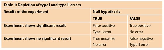
As with all statistical tests and experiments, errors are expected. The common errors related to hypothesis testing are known as type 1 and type 2 errors. A type 1 error occurs when the null hypothesis is rejected even though it is true [1,2]. This is sometimes also known as a false positive result [4]. The probability of this occurring is indicated by the significance level of the test – as explained above, the significance level of 0.05 means that there is a 5% chance that the decision to reject the null hypothesis is wrong. This is sometimes denoted as alpha (a). An example of a false positive in the clinical setting is an individual testing positive for pregnancy when they are not pregnant. A type 2 error, on the other hand, is when the null hypothesis is accepted but it is false [1]. This is also known as a false negative [4]. The probability of type 2 errors occurring is denoted as beta (ß). Type 2 errors are closely related to the statistical power of a hypothesis test; this power is defined as 1- ß. Thus, the power tells us the probability that we correctly reject the null hypothesis. Power is closely related to sample size and consequently type 2 errors tend to occur when the sample is too small. Hence, a study with a small sample size and thus low power will have a greater likelihood of a type 2 error. Typically, a power of 80% or higher is deemed appropriate for research studies and should be taken into consideration when planning a study. Table 1 depicts the circumstances under which type 1 and type 2 errors would occur [5].
Confidence intervals are another example of a helpful method in interpreting results using statistical analysis – it tells us how much uncertainty there is around a particular parameter. Say we take a sample from a population of interest; we aim to work out a mean of a specific characteristic for the people using this sample, e.g. weight. However, the selection is only a tiny chunk of the population and randomly selected; hence there is a slight chance that the mean may not be representative of the actual value. Different samples of the same population may indeed end up giving a variety of diverse values – this is known as sampling error. This is where the use of a confidence interval can be helpful. A 95% confidence interval provides a range in which the population mean could lie, with a 5% chance that this is not the case [6]. So, there is a 0.95 probability of the population mean lying within the calculated range. The larger the sample size, the lower the sampling error and the narrower the confidence interval [4]. In order to calculate the confidence interval, we must consider the standard error.
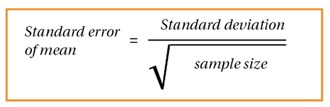
Figure 1.

Figure 2.
Simply put, the standard error is the standard deviation (please refer to part 1 for further details on standard deviation) of the means acquired from all the different possible same-size samples from the population [3]; thus, the standard error tells us the standard deviation of a population’s sampling distribution. The formula, seen in Figure 1, simply uses the population standard deviation. We then use the formula in Figure 2 to work out upper and lower values for the confidence interval. Note that ±1.96 is used to represent the z score (normal standard deviations) at ±2.5% to obtain a 95% confidence interval.
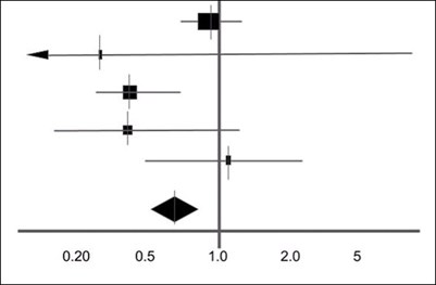
Figure 3: An example of a simple forest plot.
Confidence intervals are commonly represented through forest plots. A forest plot is frequently used to represent results from a meta-analysis [7]. These are usually a collection of results from a variety of different studies. A forest plot can concisely represent their findings. Figure 3 is an example of a forest plot obtained from a systematic review [8]. Usually, a shape in the middle represents the result of the study with the horizontal line representing the 95% confidence interval [9]. At the bottom is a shaded diamond representing the overall result from the analyses. The vertical line in the middle represents the null hypothesis where there is no significant difference. Depending on the hypothesis, if the result lies either to the left or the right of the line, the results are significant and favour either side of a two-tailed test. If the overall result is touching the vertical line, there is no significant difference [7].
Tests for comparing different types of data
Analysis of results is a critical part of statistics which allows us to make conclusions alongside calculating if the null hypothesis is to be accepted or rejected. There are a variety of different tests that enable us to make comparisons between data. One example is the t-test which is primarily used to compare means between two different groups of data. As explained above, the null hypothesis states that there is no significant difference between the two means. There are a number of distinct t-tests that can be used [9]:
- One sample t-test: one group mean is being compared to set values, e.g. average height.
- Two sample t-test: comparing two group means that have been obtained from different populations, e.g. populations from two different countries. This is also known as the Student’s T-test and is the most commonly used. Figure 4 represents this, where s2 is the standard pooled error and n represents the number in each population. The standard pooled error is the average standard error from the two populations.
- Paired t-test: comparing two group means that have been obtained from a single population, e.g. same country.
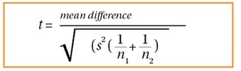
Figure 4.
What the t-test actually represents is a difference between the two means. From this, we can then obtain a P-value using probability tables, which is then used to make a conclusion whether to either accept or reject the null hypothesis.
Although practical, t-tests can only be used to compare two groups of data. However where there are greater than two groups of data, analysis of variance (ANOVA) testing can be useful and provide a solution to comparing larger groups of data that are all independent [10]. ANOVA analyses differences between the group averages through the use of the variances. Table 2 below represents what a standard ANOVA one-way table looks like, with each of the relevant formulas stated. Although this looks very daunting at first, breaking it down into each separate element makes it easier to understand.
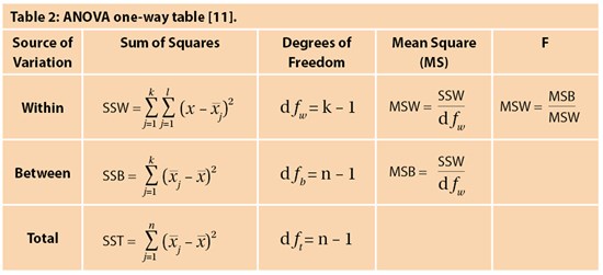
The formula for sum of squares within (SSW) represents the variation within each group, which is then all summed. This is worked out by calculating the difference between each observation in the group and the mean of that group, squaring them and taking the sum. We do this for each group and calculate the total which is SSW – this is represented by the sum function up to k (k is the number of groups). On the other hand, sum of squares between (SSB) represents variation between each of the individual groups. This is worked out by taking the difference of the group mean from the overall mean, squaring them, and summing them for the total number of groups. Finally, the total sum of squares (SST) is worked out by the addition of SSB and SSW.
Note that there is a column known as degrees of freedom. This is defined as the number of independent groups of information present; we have k-1 as the degrees of freedom as there are k sample groups but one estimated parameter from each group, which is the mean. This is also an important aspect in forming the P-value in the t-test. T
he mean squares (MS) is worked out using the degrees of freedom and the sum of squares which is very simple. We can then work out the F statistic – note that the null hypothesis states that there is no difference between the means (through using MSB and MSW), and so the F ratio is expected to be 1 if the null hypothesis is true. We again use probability tables and a significance level to obtain an F critical value to make a conclusion. In the instance that there are only two sample groups, then a t-test and ANOVA testing will give the same results.
Another method of comparing data is the chi-squared test. While the t-test is used for normally distributed parametric data, chi-squared test is non-parametric, where data follows no particular distribution [12] and assesses for relationships between categorical variables. Note that the chi-squared test is also a significance test where a hypothesis is present. The larger the value, the greater the difference between expected and observed results and the greater the chance of rejecting the null hypothesis, telling us that the variables are associated. But we still need p-values or critical values to make this conclusion. The formula for chi-squared is represented by figure 5:

Figure 5.
A much simpler formula compared to ANOVA and t-tests. We must take the difference between observed and expected values, square this, and divide by the expected value. We do this for each of different sets of observed and expected values and take the sum of this. We can then use the result to make a conclusion whether or not to reject the null hypothesis.
There are also some other tests such as Mann Whitney U and Fisher’s Exact test which can be used for hypothesis testing. Determining which type of hypothesis test to use depends on the type and distribution of the data, how many groups are being compared and the characteristics of the outcome variables. Therefore, it is always useful to contact a statistician to determine the most appropriate test for statistical analysis. Most types of hypothesis tests are commercially available or can be found in online statistical packages. It is important to remember that hypothesis tests can only give information about the statistical significance of the data but do not provide any information about the clinical significance of the result.
To conclude, this article has given an overview of probability, hypothesis testing and comparing groups of data. The third and final part of this series will focus on statistics in diagnostic testing.
References
1. Banerjee A, Jadhav SL, Bhawalkar JS. Probability, clinical decision making and hypothesis testing. Industrial Psychiatry Journal 2009;18(1):64-69.
2. Peacock JL, Peacock PJ. Oxford Handbook of Medical Statistics. Oxford, UK: Oxford University Press; 2011.
3. Harris M, Taylor G. Medical Statistics Made Easy. Oxfordshire, UK: Scion Publishing Limited; 2008.
4. Romano R, Gambale E. Statistics and Medicine – the indespensable Know-How of the Researcher. Transl Med UniSa 2013;5:28-31.
5. Shreffler J, Huecker M. Type I and Type II Errors and Statistical Power. StatPearls [Internet] 2021.
6. Hazra A. Using the confidence interval confidently. Journal of Thoracic Disease 2019;9(10):4125-30.
7. Verhagen AP, Ferreira ML. Forest plots. Journal of Physiotherapy 2014;60(3):170-3.
8. Wilt T, Ishani A, MacDonald R. Serenoa repens for benign prostatic hyperplasia [Update]. Cochrane Database Syst Rev 2002;3:CD001423.
9. Kim TK. T test as a parametric statistic. Korean Journal of Anesthesiology 2015;68(6):540-6.
10. Kim TK. Understanding one-way ANOVA using conceptual figures. Korean Journal of Anesthesiology 2017;70(1):22-6.
11. Image adapted from: https://byjus.com/anova-formula/
12. McHugh ML. The chi-square test of independence. Biochemia Medica 2013;23(2):143-9.
Declaration of competing interests: None declared.